FYBCOM Economics Sem 1 Chapter 7 Notes (Cost Concepts)
Q.1 Explain the following concepts-
a) Implicit cost and Explicit cost
Answer: Implicit cost refers to the cost of all own factors which the entrepreneur employs in the business. It includes salary and wages for the service of entrepreneur, interest on capital invested by the entrepreneur etc. Implicit costs are also called indirect cost because direct cash payment is not made to own factors of production.
If entrepreneur sold these services to others, he would have earned money. Therefore, implicit cost is also the opportunity cost of factors owned by him.
Explicit cost on the other hand is the direct cash payment made by the firm for purchasing or hiring of various factors of production. E.g. rent paid for hiring of land, money spent for
purchasing for raw material, wages and salaries paid to the employees, expenditure on transport, power, advertising etc.
b) Private cost and Social cost
Answer: Costs which are directly incurred by the individual or firm producing good or service is called private cost. This cost gives private benefit to an individual or firm engaged in relevant activity. Some of the examples of private cost are firm’s expenditure on purchase of raw material, payment of rent, wages and salaries, interest, insurance, depreciation etc.
Similarly company’s expenditure for its labor, advertising cost for the promotion of goods, transportation cost to carry goods from company to the market are also considered as private cost.
Social cost on the other hand is bared by the society as a result of production of commodity. Even though social cost occurs due to production of a commodity it is not bared by the producer. It consists of external cost. E.g.: If a factory is located in a residential area causes air pollution. Due to pollution as the health of the people living in that area affects, they have to spend money on medical facilities. Even though this cost occurs due to the factory, it is passed on to the society at large.
Externalities are included in the social cost.
c) Historical cost and Replacement cost
Answer: The original money value spent at the time of purchasing of an asset is called historical cost. Most of the assets in the balance sheet are at the historical cost. One of the advantages of historical cost is that records maintained on the basis of historical cost are
considered to be reliable, consistent, comparable and verifiable.
Historical cost does not reflect current market valuation.
The amount which has to be spent at the time of replacing of the existing asset is called the replacement cost. This cost reflects the current market prices. If we consider an increase in prices over the years, replacement cost will be greater than historical cost. If we consider fall in prices over the years, replacement cost will be less than historical cost and if we consider prices to be constant over the years, replacement cost and historical costs are the same.
d) Total cost, Average cost and Marginal cost
Answer: Total cost (TC) – Firms total expenditure on all fixed and variable factors for producing a commodity is called the Total cost of production.
Therefore TC= TFC+TVC
For zero level of output there is some total cost. It increases with an increase in the level of output.
Average Cost (AC) or Average Total Cost (ATC) – It refers to the per unit cost of producing a commodity. It is calculated by the following formula
AC = TC/Q
Where AC = Average cost TC = Total cost Q = Number of units produced
Average cost can also be calculated by using following formula- AC or ATC = AFC+AVC
Where AC – Average Cost AFC – Average Fixed Cost AVC – Average Variable Cost
Average Fixed Cost (AFC)- It is the per unit fixed cost of production. It can be calculated by the following formula
AFC= TFC/Q
Where TFC= Total Fixed Cost Q = Number of units produced
Average Variable Cost (AVC) – It is the per unit variable cost of production. It can be calculated by the following formula
AVC= TVC/Q
Where TVC= Total Variable Cost Q= Number of units produced
Marginal Cost (MC) – It is the addition made to the total cost. Or cost of producing an additional unit of output is called as the marginal cost. It can be calculated by using following formula
MC = Change in total cost/ change in output TC
Q
Where, △TC = Change in Total Cost
△Q = Change in Output
OR
MC= TCn- TCn-1
Eg: If total cost of producing 2 cars is Rs. 3, 00,000 and the total cost of producing 3 cars is Rs. 4, 50,000.
Then the marginal cost is Rs. 1, 50,000 i.e. the cost of producing an additional unit of output.
e) Fixed cost and Variable cost
Answer: Fixed cost refers to the firm’s expenditure on fixed factors of production. Even if no output is produced, fixed cost needs to be paid. Even if output increases in the short run, fixed cost remains constant.
E.g.: If a businessman borrows money from a bank to start his business. Initially even if his output is zero, he has to pay the interest on borrowed capital. Rent on land, insurance premium, tax payment are some of the examples of fixed cost. Addition of all
fixed cost gives Total Fixed Cost.
Variable cost on the other hand refers to the firm’s expenditure on variable factors of production. When no output is produced, variable cost is zero. As output increases, variable cost also increases. Payment for raw material, wages and salaries of the workers are some of the examples of variable cost. Addition of all variable costs gives the Total Variable Cost.
f) Opportunity cost
Answer: Opportunity cost (also known as “alternative cost,”) is the difference between a project’s cost estimate and another option that must be foregone in order to implement the project.
Opportunity Cost, which refers to the value of the next best alternative that must be given up when a decision is made, is a fundamental idea in economics. It draws attention to the trade-offs present in all decisions. When resources are scarce, picking one course of action over another has a cost because the resources might otherwise be employed for the alternate.
e.g: The happiness and relaxation you forfeit, for instance, if you opt to spend the evening preparing for an exam rather than seeing a movie, is the opportunity cost. To make wise decisions and utilise resources effectively, both organisations and individuals need to understand opportunity cost. It is crucial in determining the true costs and benefits of choices, assisting in resource allocation optimisation for best value.
Q.2 Explain the relationship between TFC, TVC and TC with the help of diagram.
Answer: TFC is the firm’s total expenditure on fixed factors of production. For zero level of output TFC is zero. It remains constant for all the levels of output.
TVC on the other hand is the firm’s total expenditure on variable factors of production. For zero level output TVC is zero. It increases with an increase in the level of output.
Total cost is the additional of Total Fixed Cost and Total Variable Cost.
In the following table relationship between TFC, TVC and TC is discussed for different units of output
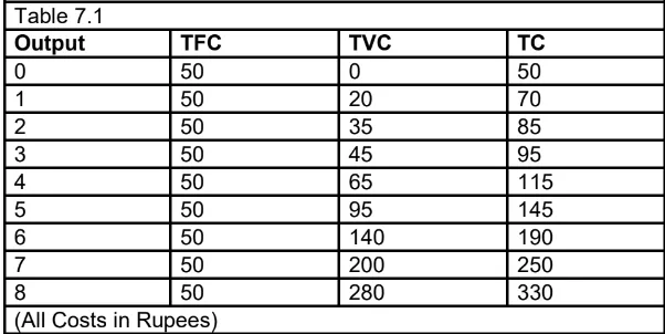
Explanation – In table 7.1 First column shows various levels of output starting from zero units to 8 units. Second column shows TFC. As fixed factors of production are constant for certain level of output TFC is also constant for all level of output. For zero level of output also TFC is Rs. 50. Third column shows TVC which is zero for zero level of output. With an increase level of output TVC initially increases at decreasing rate then increases at an increasing rate.
This is because of the law of variable proportions. Forth column shows TC which is the addition of TFC and TVC. TC increases with an increase level in the output. TC increases in the same
proportions as increased in TVC.
This relation between TFC, TVC and TC can be explained with the help of following diagram.
Two curves are parallel to each other.
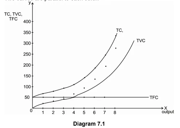
By plotting different combinations of output and TFC, TVC and TC, we have TFC curve, TVC curve and TC curves.
Diagram shows that TFC curve is a straight-line curve parallel to X axis. This is because when output is zero, some fixed cost has to be paid and this cost remains constant for all the levels
of output. TFC curve is horizontal.
TVC curve starts at the point of origin because when output is zero, TVC is also zero. TVC curve initially increases at a diminishing rate with an increase in the level of output and then
increases at an increasing rate.
As TC is the addition of TFC and TVC, TC curve is above TFC and TVC curves. The shape of TC curve is same as the TVC curve. The gap between TC and TVC curve measures TFC.
Q.3 Define AC,AFC, AVC and MC and also discuss the relationship between them.
Answer: Average Cost (AC) or Average Total Cost (ATC) – It refers to the per unit cost of producing a commodity. It is calculated by the following formula
AC = TC/Q
Where AC = Average cost TC = Total cost Q = Number of units produced
Average cost can also be calculated by using following formula- AC or ATC = AFC+AVC
Where AC- Average Cost AFC- Average Fixed Cost AVC- Average Variable Cost
Average Fixed Cost (AFC)- It is the per unit fixed cost of production. It can be calculated by the following formula
AFC= TFC/Q
Where TFC= Total Fixed Cost Q = Number of units produced Average Variable Cost (AVC) – It is the per unit variable cost of production. It can be calculated by the following formula
AVC= TVC/Q
Where TVC= Total Variable Cost Q= Number of units produced
Average Variable Cost (AVC) – It is the per unit variable cost of production. It can be calculated by the following formula
AVC= TVC/Q
Where TVC= Total Variable Cost Q= Number of units produced
Marginal Cost (MC) – It is the addition made to the total cost. Or cost of producing an additional unit of output is called as the marginal cost. It can be calculated by using following formula
MC = Change in total cost/ change in output TC
△Q
Where, △TC = Change in Total Cost
△Q = Change in Output
OR
MC= TCn- TCn-1
Relationship between AC and MC :
Average Cost (AC) is the per unit cost of production and Marginal Cost (MC) is the cost of producing an additional unit of output. Relationship between AC and MC can be discussed with the help of following diagram.
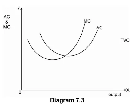
For initial levels of output AC and MC both curves are declining, but MC is less than AC.
When MC is less than AC it means that cost of producing an additional unit of output is less than per unit cost of production.
As MC<AC, new AC must be less than old AC. Therefore, AC curve is declining.
At a certain level of output (optimum level of output) AC is minimum. At this point MC curve intersects AC curve. Thus AC=MC. It means that cost of producing an additional unit of
output is exactly equal to the average cost of production. As AC=MC, new AC must be equal to the old average cost.
At higher levels of output AC and MC both are increasing but MC>AC. It means that the cost of producing an additional unit of output is greater than the average cost of production. As
MC>AC, new average cost must be greater than old average cost. Therefore, AC curve is rising.
From the above explanation we can conclude that when
- MC<AC, MC pulls the AC curve down.
- MC=AC, AC curve is flat as MC pulls AC horizontally.
- MC>AC, MC pulls the AC curve up.
- Long run cost and output relationship
As the name suggests long run refers to a sufficiently long period. As the long period is available, firm can make necessary change in all factors of production as per the changes in demand.
Thus, in long run all factors of production are variable. Hence there are no fixed cost in the long run. Depending on the type of industry the length of long run can differ. For a firm producing a particular product, long run may be years.
In the long run firm can make proper planning and build that size of plant which will minimize the cost of production for producing optimum level of output. Once the particular plant has
been built, the firm operates in the short run. This means that even though firm operates in the short run, it plans in the long run.
Q.4 Bring out the relationship between AC and MC.
Answer: Refer Question No.3
Q.5 Explain the derivation of Long run Average Cost curve.
Answer: Different plant sizes are available to the firm to operate in the long run. For a specific level of output, the plant of specific size is more suitable. For every size of plant there will be a specific average cost and thus a specific average cost curve.
In the long run different short run average cost curves are available for different sizes of plant. The firm has to choose the specific size of plant for its operation.
Derivation of Long run average cost curve with a number of short run average cost curves can be discussed with the help of following diagrams-
Here we assume that there are three sizes of plant.
Above figure shows that there are three plants available to the firm and are shown by three different cost curves- SAC1, SAC2 and SAC3. For a particular level of output, a specific plant is most suited.
Above diagram shows that for producing OQ level of output on plant SAC1, cost is BQ and on plant SAC2 cost is AQ. This shows that OQ level of output can be produced with lower cost QB
with SAC1 as compared to plant SAC2.
If the firm wants to produce OQ1 level of output, it can be produced either with plant SAC1 or SAC2. But it is better for the firm to go with plant SAC2 because as shown in the diagram higher level of output OQ2 can be produced with much lower cost on SAC2. With plant SAC2, output greater than OQ1 and less than OQ3 can be produced at lower average cost.
For output greater than OQ3 firm will use plant SAC3 because the average cost with SAC2 will be greater as compared to average cost with SAC3.
Derivation of LAC

From the above explanation it is clear that in the long run the firm has alternative plant sizes available for the production and the firm will choose that plant size which gives minimum average cost for producing a given level of output. Accordingly ( Fig 7.4) with three short run average cost curves the Long run Average Cost curve is HBCEGI.
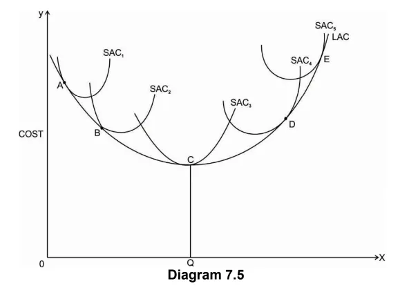
If we assume that there are infinite plant sizes available, there are number of short run average cost curves corresponding to each plant size. Therefore, the LAC will be a smooth U–shaped curve as shown in (Diagram 7.5) above.
As LAC curve is a locus of points of the lowest average cost of producing different levels of output. Every point of LAC will have a tangency point with SAC curve. It can be seen from the above diagram that LAC curve is tangent to the minimum point of SAC3 curve only at the optimum level of output OQ. Plant SAC3 is considered as the optimum size of plant because it produces optimum level of output OQ with minimum cost CQ.
For any output less than OQ, LAC curve is tangent to SAC curve on its declining part ie. at point A and B on SAC1 and SAC2.
For any output greater than OQ, LAC curve is tangent to SAC curve on its increasing part i.e. At point D and E on SAC4 and SAC5.
It can be seen from (Diagram 7.5) that LAC curve initially declines, reaches to minimum and again increases with an increase in the level of output. LAC curve is much flatter than SAC curves. LAC curve declines due to economies of scale and increases due to diseconomies of scale.
As the LAC curve includes the family of short run average cost curves, it is called an Envelop curve. In the long run firm can also plan to increase its scale of production and therefore LAC
curve is also called the Planning Curve.
Q.6 Discuss the Learning curve effect.
Answer: The learning curve shows an inverse relationship between an average cost of production and the level of output. This means that as firm produces more and more output, its average cost of production declines. Therefore, the learning curve slopes downward from left to right. Following diagram explains the learning curve effect.

In the above diagram X axis represents total output and Y axis represents the average cost. It shows that average cost is RS.6000 for producing 10 units of output. As output increases to 20, 30 and 40 units, average cost declines to 4000, rs. 3000 and rs. 2000 respectively. Points P, Q, R and S shows different combinations of output and average cost.
Learning curve effect is a result of an experience which the firm gains during the process of production. When the firm is new, it takes time for the firm to produce the output. Thus, the costs are high. As firm becomes older, it learns to use new techniques of production, efficient way of using raw material and skills. Workers also become efficient over a period of time. All this will help to reduce the average cost of production. Firm learn to reduce cost through experience. Therefore, learning curve is also called an Experience curve. The effect of learning curve applies to the manufacturing and service sector.
As shown in the diagram learning curve initially declines faster and then declines at a slower rate. This means that when the production process is new, average cost declines much faster as compared to the old production process.
Q.7 If the Total fixed cost of production is rs.75, with the help of following data, calculates TC, AC, AFC, AVC, MC.
| Output | 0 | 1 | 2 | 3 | 4 | 5 |
| TVC | 0 | 35 | 50 | 70 | 100 | 160 |
Pingback: FYBCOM Economics Sem 1 Chapter 4 Notes | FYBAF | FYBMS | Mumbai University - University Solutions
Pingback: FYBCOM Economics Sem 1 Chapter 5 Notes | FYBAF | FYBMS | Mumbai University - University Solutions
Pingback: FYBCOM Economics Sem 1 Chapter 8 Notes | FYBAF | FYBMS | Mumbai University - University Solutions
Pingback: FYBCOM Economics Sem 1 Chapter 1 Notes | FYBAF | FYBMS | Mumbai University - University Solutions
Pingback: FYBCOM Sem 1 Basic Tools in Economics Chapter 1 Notes 2024 | FYBAF | FYBMS - Mumbai University - University Solutions
Pingback: FYBCOM Sem 1 Basic Tools in Economics Chapter 3 Notes 2024 | FYBAF | FYBMS - Mumbai University - University Solutions
Pingback: FYBCOM Sem 1 Basic Tools in Economics Chapter 5 Notes 2024 | FYBAF | FYBMS - Mumbai University - University Solutions
Pingback: FYBCOM Sem 1 Basic Tools in Economics Chapter 6 Notes 2024 | FYBAF | FYBMS - Mumbai University - University Solutions