FYBCOM Economics Sem 1 Chapter 8 Notes
(Extension of Cost Analysis)
Q.1) Select the correct answer from the alternatives given and rewrite the sentences:
1) At the break-even point, the price is equal to _______ cost.
a) Total
b) Marginal
c) Average
d) Variable
2) At the shutdown point, price is equal to average _______ cost.
a) Fixed
b) Variable
c) Above
d) Below
3) When the fixed cost level of output.
a) Falls
b) Rises
c) Remains constant
d) Shfits down
4) The shutdown and break-even points are the break-even point _____.
a) Same
b) Different
c) Irrelevant
d) Equal
5) Break-even point is reached when a firm .
a) earns zero profit
b) covers fixed cost
c) covers variable cost
6) A firm is at break even point when
a) TR > TC
b) TR < TC
c) TR = TC .
7) A break-even point changes whenever there is change in
a) Price
b) Fixed cost
c) Variable cost
d) AIl three factors
8) Break-even point is easily worked out in case of a
a) Joint-product firm
b) Multiple-products firm
c) Single product
9) A firm earns Supernormal profit when its
a) TR = TC
b) TR > TC
c) TR < TC
Q.2) Answer the Following Questions
1) Explain the concept of break-even point with the help of diagram.
Answer: Break-even analysis studies the relationship between total cost, total revenue, total profits and losses over a range of output.
Break-even point is a point where the total revenue of the firm is equal to total cost.
Therefore, at break-even point there is no profit, no loss.
Break-even analysis technique is used in the business to determine the level of production or sales volume which is necessary for the business to cover its cost of doing a business.
In financial analysis the concept of break-even point is most commonly used.
The concept of break-even point can be explained with the help of following.
| Output | TR | TC | Profit/ Loss |
| 0 | 0 | 1200 | -1200 |
| 1 | 1000 | 1500 | -500 |
| 2 | 1400 | 1800 | -400 |
| 3 | 2000 | 2000 | 0 |
| 4 | 2600 | 2200 | 400 |
| 5 | 3500 | 3000 | 500 |
Above table shows that break-even level of output is 3 units because, firms TR and TC are equal at 3 units of output and therefore there is no profit, no loss.
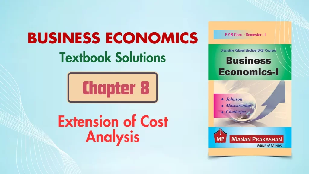
Break-even point can also be explained with the help of following diagram
Above diagram is drawn on the basis of the assumption that TR and TC curves are linear i.e. TR and TC increases at a constant rate with an increase in the level of output. Therefore, TR and TC curves are straight lines.
For initial levels of output total cost is greater than total revenue therefore the firm is making loss. At output OQ, firm stops making loss, TR=TC therefore there is no profit no loss. Thus, OQ
is the break-even output and B1 is the break-even point. After OQ level of output total revenue is greater than total cost and thus firm starts making profit.
When TR and TC curves are linear, there is only one break-even point. According to above diagram entire output after break-even output gives profit. However, this may not be true because of changes in price and cost.
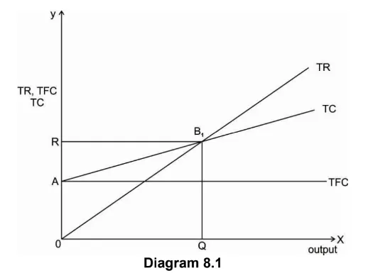
If we do not consider constant change in TR and TC, TR and TC curves are non-linear.
In this case we have more than one break-even point as shown in the following diagram-
In the above diagram on the Y axis we measure cost and revenue and on the X axis
we measure output.
In case of non-linear TR and TC curves there two break-even points P and Q, indicating lower level of output OM and higher level of output ON respectively.
For any output less than OM and greater than ON, firm makes losses because TC>TR.
Between the range of output M and N, TR>TC and thus firm makes profit.
2) Discuss with the help of diagram how break-even point changes due to change in price and fixed cost.
Answer: Any change in price will have an effect on total revenue and therefore also on break-even point. If we consider the same example 1 and consider an increase in price to Rs.17, and keep fixed cost and average variable cost constant, break-even quantity is-
QB = FC/ P-AVC
= 4000/17-7
= 4000/10
= 400 units.
If we consider fall in price to Rs. 12, keeping fixed cost and average variable cost constant, break-even quantity is-
QB = FC/P-AVC
= 4000/12-7
= 4000/5
= 800 units.
This shows that with an increase in price, break-even quantity falls and with a fall in price, break-even quantity increases.
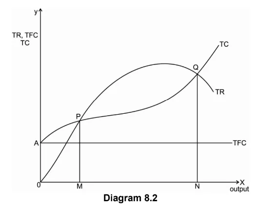
Effect of changes in price on break-even point and break-even quantity can be explained with the help of following diagram.
In the above diagram X axis measures output and Y axis measures cost and revenue. With an initial TR and TC curves A is the break-even point, where TR and TC curves intersects.
If price increases, TR curve shifts upward from TR to TR1. This will bring down the break-even point from A to A1.
Similarly, with a fall in price, TR curve shifts downward to TR2 and thus break-even point also shifts to A2.
- Changes in fixed cost
For the same mathematical example 1 if we change the fixed cost and keep price and average variable cost constant, we have changes in breakeven quantity.
Suppose fixed cost increases to Rs. 5000, break-even quantity is-
QB = FC/P-AVC
= 5000/15-7
= 5000/8
= 625 units.
If fixed cost falls to Rs. 3600, break-even quantity is-
QB = FC/P-AVC
= 3600/15-7
= 3600/8
= 450 units.
This shows that with an increase in fixed cost, break-even quantity increases and with a fall in fixed cost, break-even quantity falls.
Changes in break-even point due to changes in fixed cost can be explained with the help of following diagram-
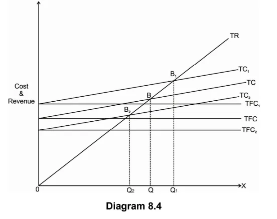
On the X axis we measure output and on the Y axis we measure cost and revenue. With an initial TR and TC curves initial break-even point is B initial break even quantity is OQ if fixed cost increases, TFC curve shifts upward to TFC1. As total cost is the addition of TFC and TVC, TC curve will also shift upward to TC1.
This shifts the break-even point at higher level to B1. Break even quantity has also increased from OQ to OQ1.
On the other hand, if TFC falls, TFC curve will shift downward to TFC2. This will shift the TC curve down to TC2.
Therefore, new break-even point is B2 & new break even quantity falls from OQ to OQ2.
3) Explain changes in break-even point due to change in total variable cost.
Answer: if TFC falls, TFC curve will shift downward to TFC2. This will shift the TC curve down to TC2.
Therefore, new break-even point is B2 & new break even quantity falls from OQ to OQ2.
- Changes in variable cost per unit
Using the same mathematical problem if we keep price and fixed cost constant and change the variable cost per unit, we have a change in break-even quantity.
Suppose the average variable cost per unit increases to Rs. 10, break-even quantity is
QB = FC/P-AVC
= 4000/15-10
= 4000/5
= 800 units.
If variable cost per unit falls to Rs. 5, break-even quantity is
QB = FC/P-AVC
= 4000/15-5
= 4000/10
= 400 units.
This shows that with an increase in per unit variable cost, break-even quantity increases and with a fall in average variable cost, break-even quantity falls.
This can be discussed with the help of following diagram-
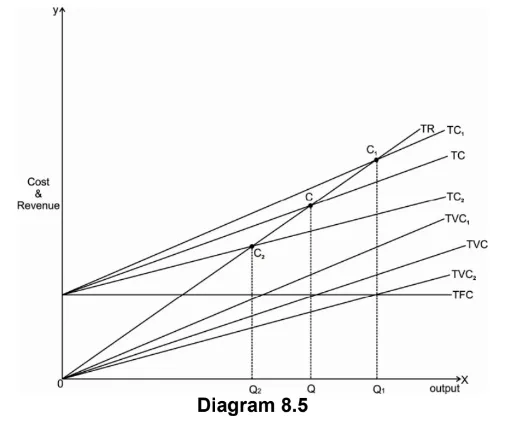
In the above diagram X axis measures output and Y axis measures cost and revenue. Initial break-even point is C where TR and TC curves intersect. Initial break even quantity is OQ. With an increase in TVC, TVC curve shifts to TVC1.
This also shifts TC curve to TC1. TVC1 and TC are parallel to each other. Thus, the
new break-even point shifts upward to C1 & break even quantity increases from OQ to OQ1.
With a fall in TVC, TVC curve shifts to TVC2, shifting down TC curve to TC2. Thus, the new break-even point also shifts down to C2. Again, TVC2 and TC2 are parallel to each other. New break even quantity falls from OQ to OQ2.
4) Discuss the implications and limitations of break-even analysis.
Answer: Linear TR and TC curves gives wrong impression that the entire output after break-even point is profitable. But this is not always true.
In case of single product unit, break-even analysis can be applied. But in case of multiple or joint products it is difficult to apply break-even analysis as long as cost cannot be determined
for each of the product.
The data required for break-even analysis including costs, price etc. is generally historical.
If historical data is not proper for estimating future costs and prices, break-even analysis cannot be usefully applied.
If it is possible to clearly classify costs as fixed and variable costs, break-even analysis is more useful. But sometimes it is not possible to have such classification of costs.
Even though there are various limitations of break-even analysis, it is useful in production planning if proper data is obtained.
Pingback: FYBCOM Economics Sem 1 Chapter 4 Notes | FYBAF | FYBMS | Mumbai University - University Solutions
Pingback: FYBCOM Economics Sem 1 Chapter 5 Notes | FYBAF | FYBMS | Mumbai University - University Solutions