FYBCOM Economics Sem 1 Chapter 5 Notes
(Supply and Production Decisions)
1) Explain the law of variable proportion in detail.
Answer: The law of variable proportion is a short run production function theory. This law plays a very important role in the economic theory, which examines the production function with which one variable factor keeping the other factors input fixed. This law is explained by the classical economists to explain the behaviour of agricultural output.
Alfred Marshall, had discussed the law in relation to agriculture, according to him, “an increase in the capital and labour applied in the cultivation of land causes in general a less than proportionate increase in the amount of product raised unless it happens to coincide with an improvement in the art of agriculture”.
Marginal productivity of labour in agriculture is zero.
Assumptions: The law of variable proportion is based on the following assumptions:
a) The state of technology is assumed to be given and constant.
b) There must be some inputs whose quantity must be kept as fixed or constant. Such input factors are called fixed factors.
c) All units of variable factors inputs are homogenous.
d) The law is based upon the possibility of varying the proportions in which the various factors can be combined to produce the level of output. Let us assume the labour is the variable factor in our explanation.
Change in output due to increase in variable factors can be explain with the table given below:
| Units of Variable factor (LABOUR) | Total Product (TP) | Average Product (AP) | Marginal Product (MP) |
| 0 | 0 | 0 | – |
| 1 | 5 | 5 | 5 |
| 2 | 12 | 6 | 7 |
| 3 | 27 | 9 | 15 |
| 4 | 48 | 12 | 21 |
| 5 | 75 | 15 | 27 |
| 6 | 80 | 13.33 | 15 |
| 7 | 91 | 13 | 11 |
| 8 | 98 | 12.5 | 7 |
| 9 | 98 | 10.8 | 0 |
| 10 | 92 | 9.2 | -6 |
Explanation of the table:
In the above table the labour is consider as a variable factor and all other factors are assumed to be constant according to the law. With the increase in the variable factor
i.e. labour there is a change in the level of TP, AP, and MP.
Total product: The total product is the total amount of output produced by using all the variable input in a fixed proportion in production. The total product increases with the increase in the unit of labour and reaches to the maximum and they’re after decline with further more increase in the variable factor.
Average product: The average product is the per unit of product produced by the firm with the per unit of variable factor inputs. It is obtained by dividing the total product by the unit of total variable factor. The average product increases initially and then declines.
Marginal product: Marginal product is the additional output produced by an additional unit of variable factor. Marginal product
increases and thereafter falls when TU becomes maximum MU becomes zero and further becomes negative.
Diagram: the law of diminishing marginal returns can be explained with the following diagram:

The above diagrams show three phases with the changes in the output can be explained below:
Phase 1: In phase 1 the total product is increasing at increasing rate where average product is also increases at a diminishing rate
and reaches at its maximum and marginal product increases initially and then decreases.
Phase 2: In phase 2 the total product increases at a diminishing rate and reaches its maximum point. Where the average product is starts declining and the marginal product diminishes and become zero.
Phase 3: In this phase total product starts declining. Where average product is continuously declining and marginal product
becomes negative.
2) Explain the law of returns to scale.
Answer: As the law of variable proportion is a short run production function theory, law of returns to scale is a long run production function theory. In this theory all factors of production are variable no factors are fixed. With the change in the factors of production scale of production will change accordingly.
According to Koutsoyiannis “The term returns to scale refers to the changes in output as all factors change by the same proportion.”
According to Koutsoyiannis
Types of return to scale: The concept of returns to scale assumes only two factors of productions i.e. capital and labour this analysis enables us to understand the change or scale in production due to change in the factors of production in terms of isoquants or equal product curves.
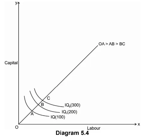
1) Increasing returns to scale: Increasing returns to scale means an increase in a level of output more than the increase in the inputs.
For example, if an output increases by 35% with an increase in all inputs by only 15% increasing returns to scale prevails. In other words, a proportionate change in output brings about less proportionate change in inputs it is called increasing returns to scale. Where, OA>AB>BC.
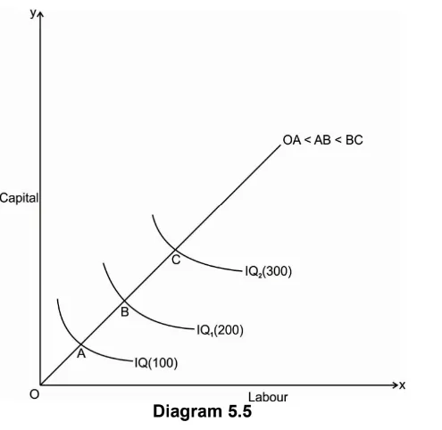
2) Decreasing returns to scale: Decreasing returns to scale means an increase in a level of output less that the increase in the inputs.
For example, if an output increase by 25% with an increase in all inputs by 35% decrease in returns to scale prevails. In other words, a proportionate change in output brings more proportionate change in inputs it is called decreasing returns to scale. Where OA<AB<BC.
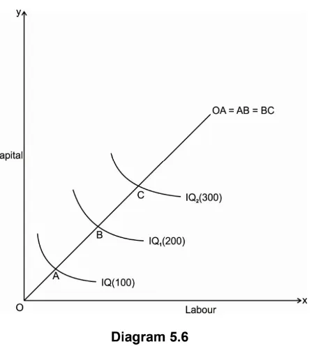
3) Constant returns to scale: Constant returns to scale means an increase in a level of output is constant that the increase in the inputs. For example, if an output increase by 25% with an increase in all inputs by 25% constant in returns to scale prevails. In other words, a proportionate change in output brings constant change in inputs it is called constant returns to scale. Where OA=AB=BC.
3) What is isoquant? Discuss its properties in detail.
Answer: The term “iso-quants” is derived from Greek word iso means “equal” and quants means “quantity”. Thus, iso-quant means equal quantity.
The isoquants have its properties which are similar to those generally assumed for indifference curve theory of the theory of consumer’s behaviour analysis. Iso-quant is defined as “a locus of all the combination of two factors of production that yields that yield the same level of output.”
Thus, an iso-quant is a combination of any two factor inputs that represents and produce the same level of output. Any two combinations of input factors e.g. Labour and capital are used in which one factor is increased by decreasing the other factor of input to maintain the same level of production.
Iso-quant can be explained with the schedule and graph given below:
Factor combinations to produce a given level of output.
| Factor combinations | Labour | Capital | Output |
| A | 1 | 150 | 500 |
| B | 2 | 100 | 500 |
| C | 3 | 75 | 500 |
| D | 4 | 50 | 500 |
| E | 5 | 25 | 500 |
There are 5 Properties of Iso-Quants which has been explained below:
1) Iso-quant curve slopes downwards:
The iso-quant curve slopes downwards from left to right i.e. it has a negative slope. The slope is downward because it operates under law of MRTS, when we increase labour as a factor, we have to decrease capital factor to produce a same level of output. The downward sloping iso-quant curve can be explaining the help of following Diagram 5.9.
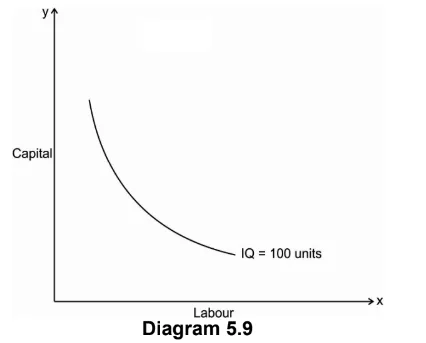
Thus, the iso-quant can be downward sloping from left to right. There can’t be an upward sloping iso-quant curve because it shows that a given product can be produce by using less of both the input factor.
Similarly, an iso-quant cannot be horizontal or vertical because it also doesn’t represent the equilibrium position of a firm. Only the downward sloping supply curve represents the characteristics of iso-quant.
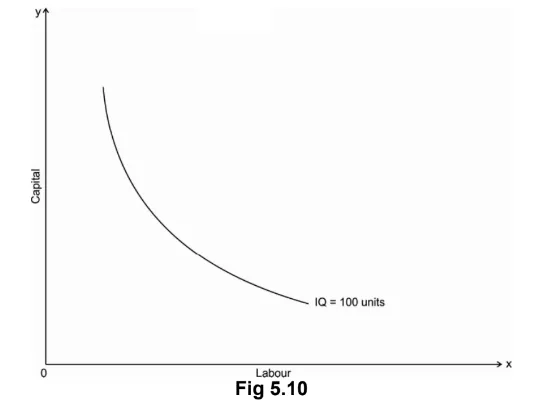
2) Iso-quant are convex to the origin:
As we had discussed in the above property that the iso-quant curve is downward sloping and it has a negative slope and it operates under law of Marginal rate of Technical Substitution (MRTS). It says that it equals the ratio of the marginal product if labour and marginal product of capital i.e. one factor is given up to get one additional unit of other factor to produce the same of output which creates a convexity of iso-quant curve.
Thus, the slope of iso-quant can be represented by,
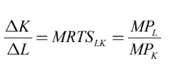
The above equation represents ratio of change in capital and labour should be equal to the ratio of the marginal rate of technical substitution of labour and capital which is equal to the ratio of marginal product of labour and capital.
The convexity of iso-quant means that as we move down the curve less and less of capital given up for an additional unit of labour so to produce the same level of output. The convexity of iso-quant can be observed from the Diagram 5.10. Given below
3) Iso-quants do not intersect:
The properties of iso-quants say that two iso-quant will never intersect each other. To explain this,
we will take a help of following Diagram 5.11:
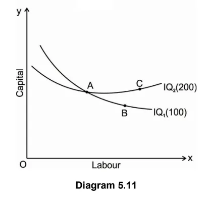
The above fig represents two different iso-quant IQ1and IQ2, where it represents the level of output 100 and 200 units respectively. Point a represents 100 units of output on IQ1 and point c represents 200 units of output on IQ2. The point b shows the intersection of both the iso-quants where is logically not possible to identify the level of output.
4) Iso-quant cannot touch either of the axis:
An iso-quant cannot only touch x axis or y axis or any either axis because it will represent that the iso-quant only produce goods by using one factors of production either by using only capital or only labour which is practically not possible and which is unrealistic.
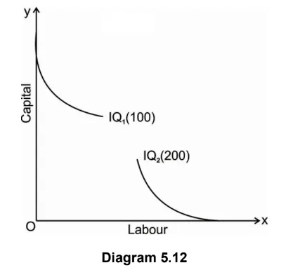
5) Higher the iso-quant higher the level of production:
if there is a multiple iso-quant showing different level of production in one diagram. Where the higher the iso-quant i.e. the iso-quant far from the origin indicates higher level of output and the iso-quant close to the origin indicates lower level of output.
4) Define isoquant. Explain the different types of isoquants.
Answer: The term “iso-quants” is derived from Greek word iso means “equal” and quants means “quantity”. Thus, iso-quant means equal quantity.
Iso-quant is defined as “a locus of all the combination of two factors of production that yields that
yield the same level of output.”
An iso-quant is a combination of any two factor inputs that represents and produce the same level of output. Any two combinations of input factors e.g. Labour and capital are used in
which one factor is increased by decreasing the other factor of input to maintain the same level of production.
The following are the various types of iso-quant based on the degree of substitutability of substitution:
1) Liner iso-quant: if the iso-quant is liner one i.e. downward sloping straight line it assumes that there is a perfect substitutability of the factors of productions. It means that capital and labour can be easily substitute from each other. i.e. the rate at which labour can be substituted for capital in production (i.e. MRTSLK) is constant. This can be seen from the following Diagram 5.14 given
below:
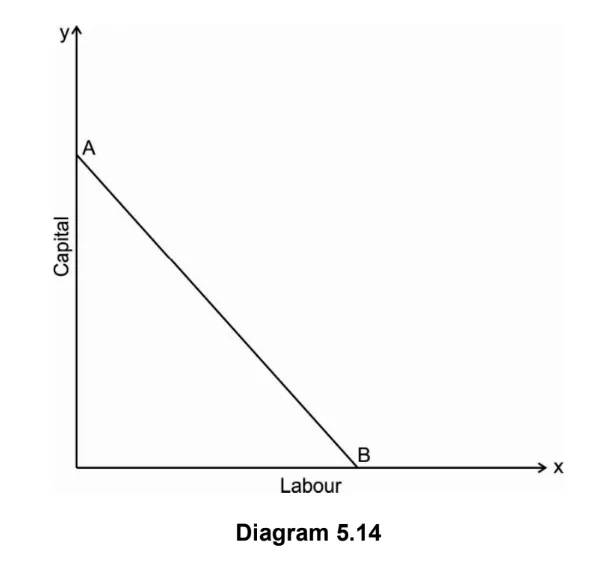
The above diagram shows that there is a perfect substitutability of labour and capital at the points A & B where point A on iso-quant represents the level of output can be produce with capital alone i.e. without using any labour on the other hand point B represents the same level of output can be produce with labour alone
i.e. without any use of capital. This in reality is not possible because no production can be done with using any of the factor alone.
2) Right angled iso-quant: if the iso-quant is right angled it assumes that there is a perfect complementarily i.e. it assumes that there is a perfect substitutability of factors of production. This shows that there is only one method is used for production of the commodity. In this type the iso-quant is formed as right angled as shown in the following fig. which shows labour and capital are used in a fixed proportion i.e. output can be increased by increasing labour and capital in fixed proportion. This type of iso-quant is known by many names such as input-output iso-quant and Leontief iso-quant.

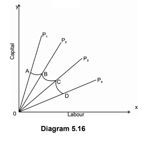
3) Kinked iso-quant: This type of iso-quant assumes only limited substitutability only at the kinked of the iso-quant. That means the substitutability of labour and capital is only possible at the kinked of the iso-quant in the production. i.e. in the fig. the substitutability is possible at the point A, B, C and D. This type of iso-quant is also called as ‘liner programming iso-quant” and it is used in liner programming.
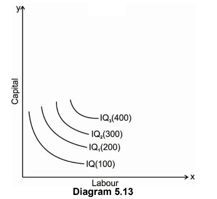
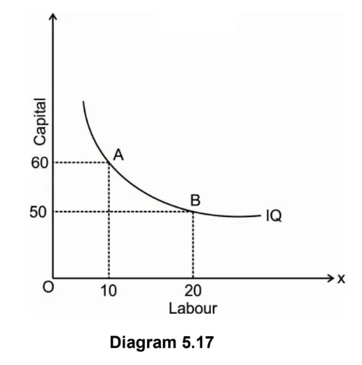
4) Smooth convex iso-quant: The classical economic theory has adopted this type of iso-quant for analysis as its simpler to understand. This iso-quant assumes the continuous substitutability of labour and capital over a certain range beyond which there is zero substitutability of factors in production. This iso-quant fulfils all the criteria of iso-quant. The derivation of this smooth convex iso- quant is explained below:
To explain the derivation of iso-quant we assume that there is a various combination of factor inputs of labour and capital used to produce 100 units of output. The combination is a such where
one factor is increased by reducing the other factor input to produce the same level of output in production. All this combination is technically efficient in production.
Various combinations of labour and capital to produce 100 units of output.
| Factor combination | Labour | Capital |
| A | 10 | 60 |
| B | 20 | 50 |
| C | 30 | 40 |
| D | 40 | 30 |
If we plot all this combination on a graph, we obtain an IQ curve.
5) Write a short note on Ridge lines.
Answer: The ridge lines are the locus of points of an iso-quants where the marginal product of factors is zero. An isoquant is oval- shaped as shown in diagram but its area of rational operation lies between the ridge lines.
The firm will produce only in those segments of isoquants which are convex to the origin and lie
between the ridge lines. The ridge lines are the locus of points of isoquants where the marginal products (MP) of factors are zero. The upper ridge line implies zero MP of capital and the lower ridge line implies zero MP of labour. Production techniques are only efficient inside the ridge lines. The marginal products of factors are negative and the methods of production are inefficient outside the ridge lines.
The ridge lines can be explained through the help of following diagram:
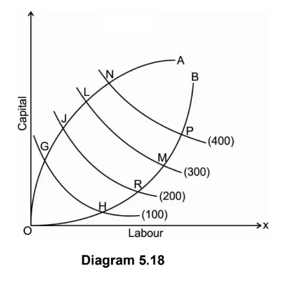
In the above Diagram curves ОA and OB are the ridge lines on the oval-shaped iso-quants and in between these lines on points G, J, L and N and H, К, M and P economically feasible units of capital and labour can be employed to produce 100, 200, 300 and 400 units of the product.
For example, ОТ units of labour and ST units of the capital can produce 100 units of the prod-uct, but the same output can be obtained by using the same quantity of labour ОТ and less quantity
of capital VT. Thus, only an unwise producer will produce in the dotted region of the iso-quant 100.
The dotted segments of isoquants form the uneconomic regions of production because they require an increase in the use of both factors with no corresponding in-crease in output.
If points G, J, L, N, H, К, M and P are connected with the lines OA and OB, they are the ridge lines. On both sides of the ridge lines, it is uneconomic for the firm to produce while it is economically feasible to produce inside the ridge lines.
6) Write a short note on Expansion path.
Answer: Expansion path is also called scale line. The expansion path is so called because if the firm decides to expand its operations, it would have to move along this path. The expansion path in simple word is defined as the locus of the points of tangency between the isoquants and iso-cost lines. The expansion paths show how a business firm tries to expand his output in the long run with the
given factor prices and the given various factor combinations.
This can be explained with the following diagram given below:
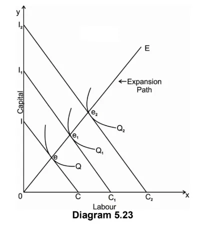
Explanation of the diagram:
X axis examines Labour and Y axis Capital. IC, I1C1 and I2C2 are the iso-cost line parallel to each other which shows factor prices are assumed to be constant. Q, Q1 and Q2 are the Iso-
quant. ‘e’ is the point of tangency which shows a firm can produce Q level quantity of output with least cost and least combination of factors of production.
Similarly, if firms want to increase his level of output, he will be on point e1 and point e2 for the maximum level of output at minimum cost and minimum level of factor inputs.
If we join all this tangency point E, E1 and E2 we will get a line OE called as expansion path or scale line. It is important to note that at the tangency point e, e1 and e2 the marginal rate of technical
substitution of labour for capital is equal to the ratio of factor prices.
Expansion path helps the business firm to find the cheapest way to produce each level of output with given factor price. It helps the firm to produce those level of output with the least cost and by using the least factor combination of input.
7) Write a short note on Producers behaviour.
Answer: Producer behavior is the actions, decisions, and strategies of firms in the marketplace, focusing on production decisions, resource allocation, pricing strategies, market entry and exit, market competition, price elasticity of supply, profit maximization, government regulations, market signals, and risk management.
Producers must decide what and how much to produce, allocate resources, and choose efficient production methods influenced by factors like costs, technology, and market demand. They also make decisions on market entry and exit, assessing market conditions, potential profitability, competition, and risks.
Producers also consider the price elasticity of supply, which measures responsiveness to price changes. They aim to maximize profit by balancing revenue and costs, complying with government regulations, and adapting to market signals. Risk management strategies include diversification, insurance, and contingency planning.
Pingback: FYBCOM Economics Sem 1 Chapter 4 Notes | FYBAF | FYBMS | Mumbai University - University Solutions
Pingback: FYBCOM Economics Sem 1 Chapter 6 Notes | FYBAF | FYBMS | Mumbai University - University Solutions
Pingback: FYBCOM Economics Sem 1 Chapter 1 Notes | FYBAF | FYBMS | Mumbai University - University Solutions
Pingback: FYBCOM Economics Sem 1 Chapter 2 Notes | FYBAF | FYBMS | Mumbai University - University Solutions
Pingback: FYBCOM Economics Sem 1 Chapter 3 Notes | FYBAF | FYBMS | Mumbai University - University Solutions
Pingback: FYBCOM Sem 1 Basic Tools in Economics Chapter 1 Notes 2024 | FYBAF | FYBMS - Mumbai University - University Solutions
Pingback: FYBCOM Sem 1 Basic Tools in Economics Chapter 2 Notes 2024 | FYBAF | FYBMS - Mumbai University - University Solutions
Pingback: FYBCOM Sem 1 Basic Tools in Economics Chapter 3 Notes 2024 | FYBAF | FYBMS - Mumbai University - University Solutions
Pingback: FYBCOM Sem 1 Basic Tools in Economics Chapter 4 Notes 2024 | FYBAF | FYBMS - Mumbai University - University Solutions
Pingback: FYBCOM Sem 1 Basic Tools in Economics Chapter 6 Notes 2024 | FYBAF | FYBMS - Mumbai University - University Solutions