
FYBCOM Economics Sem 1 Chapter 2 Notes
(Demand Analysis)
1) Explain the law of demand and the factors with determines the demand.
Answer : The law of demand was introduced by Prof. Alfred Marshall in his book, ‘Principles of Economics’, which was published in 1890. The law explains the functional relationship between price and quantity demanded.
Statement of the Law: According to Prof. Alfred Marshall, “Other things being equal, higher the price of a commodity, smaller is the quantity demanded and lower the price of a commodity, larger is the quantity demanded.”
In other words, other factors remaining constant, if the price of a commodity rises, demand for it falls and when price of a commodity falls demand for the commodity rises. Thus, there is an inverse relationship between price and quantity demanded. Symbolically, the functional relationship between demand and price is expressed as :
Determinants of Demand
The demand for goods is determined by the following factors.
1) Price: Price determines the demand for a commodity to a large extent. Consumers prefer to purchase a product in large quantities when price of a product is less and they purchase a product in small quantities when price of a product is high.
2) Income: Income of a consumer decides purchasing power which in turn influences the demand for the product. Rise in income will lead to a rise in demand for the commodity and a fall in income will lead to a fall in demand for the commodity.
3) Prices of Substitute Goods: If a substitute good is available at a lower price then people will demand cheaper substitute good than costly good. For example, if the price of sugar rises then demand for jaggery will rise.
4) Price of Complementary Goods: Change in the price of one commodity would also affect the demand for other commodity. For example, car and fuel. If the price of fuel rises, then demand for cars will fall.
5) Nature of product: If a commodity is a necessity and its use is unavoidable, then its demand will continue to be the same irrespective of the corresponding price. For example, medicine to control blood pressure.
6) Size of population: Larger the size of population, greater will be the demand for a commodity and smaller the size of population smaller will be the demand for a commodity.
7) Expectations about future prices: If the consumer expects the price to fall in future, he will buy less in the present at the prevailing price. Similarly, if he expects the price to rise in future, he will buy more in the present at the prevailing price.
8) Advertisement: Advertisement, sales promotion scheme and effective salesmanship tend to change the preferences of the consumers and lead to demand for many products. For example, cosmetics, toothbrush etc.
9) Tastes, Habits and Fashions: Taste and habits of a consumer influence the demand for a commodity. If a consumer likes to eat chocolates or consume tea, he will demand more of them. Similarly, when a new fashion hits the market, the consumer demands that particular type of commodity. If a commodity goes out of fashion then suddenly the demand for that product tends to fall.
10) Level of Taxation: High rates of taxes on goods or services would increase the price of the goods or services. This, in turn would result in a decrease in demand for goods or services and vice-versa.
2) Explain the nature of demand curve under different markets.
Answer: Economist have classified the various markets prevailing in a capitalist economy into :
a) Perfect competition
b) Monopolistic competition
c) Oligopoly
d) Monopoly
“Economist understand by the term market not any particular market place in which things are bought and sold but the whole of any region in which buyers and sellers are in such free interaction with one another that the price of the same good tends to equality easily and quickly’’.
According to Cournot, a French economist
The type of different market depends on number of factors. Accordingly, the nature of demand curve is different in different market. The nature of demand curve under various market structure are as follows:
a) Demand Curve in Perfect Competition:
Perfect competition is said to prevail when there are large number of producers (firms) producing and selling homogenous product.
The maximum output produce by the individual firm is very small relatively to the total demand to the industry product so that firm cannot affect the price by varying its supply of output.
The seller is the price taker he accepts the price determined in the market by market demand and market supply. Thus, the individual price under perfect competition is determine by the market demand and market supply.
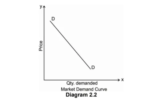
i) Market Demand Curve: The market demand curve under perfect competition is downward sloping. Because price and quantity demand are inversely related to each other as the price of a commodity increases the demand for that good decreases. The market price at which the firms will sell their commodity is determined by the interaction of market demand and market supply.
Once the market determines the price for the commodity all firms will fix their price equals to market price as they are price taker under the perfect competition. Thus, the individual demand curve is equal to the equilibrium price of the market.
The Diagram 2.2. shows the market demand curve which is downward sloping and P0 is the equilibrium market price which is followed by all the individual firm and the individual firm is facing the horizontal demand curve.
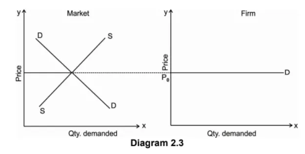
ii) Individual firm demand curve: Demand curve facing an individual firm working under prefect competition is perfectly elastic
i.e. a horizontal straight line parallel to X axis at a given price which is determined by the market demand sand market supply.
The Diagram 2.3 shows Qty demanded on X axis and Price of the commodity on Y axis. Where OP1 is the price determined by the
interaction of market demand and market supply curve. It shows if firm tries to lower the price, he will get negative profit.
b) Demand Curve under Monopoly: Monopoly is a market where there is single firm producing and selling product which has no close substitute. As being the single seller, monopoly has a control on supply and he can also decide the price of a commodity. But however, a rational monopolist who aim at maximum profit will control either price or supply. As monopolists is the only single seller in the market, he constitutes the whole industry. Therefore, the demand curve under monopoly market is downward sloping and has a steeper slope as shown in the Diagram 2.4. below:
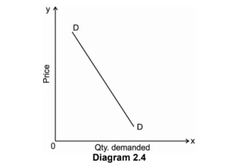
Thus, in monopoly there is a strong barrier to entry new firm in the industry. If the monopolist firm wants to increases the sale in
the market, he has to lower the price of its commodity.
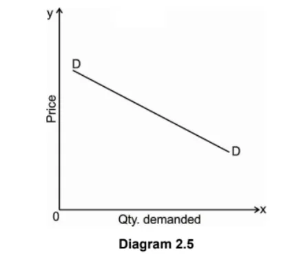
c) Demand curve under Monopolistic Competition: In the monopolistic market there is a large number of firms producing or selling somewhat differentiated product which have close substitute. As a result, demand curve facing a firm under monopolistic competition is sloping downward and has a flatter shape which is highly elastic and this indicate that a firm enjoy some control over the price of a commodity. The demand curve facing an individual firm under monopolistic competition is shown in the following Diagram 2.5.
d) Demand curve under Oligopoly Market : Oligopoly is a market where there are few firms or sellers producing or selling differentiated products. The fewness of firm ensures that each of them will have some control over the price of the product and the demand curve facing each other will be downward sloping which indicates the price elasticity of demand for each firm will not be infinite. As there are interdependence of firm. Any decision regarding change in the price of output attracts reaction from the rival firms. Therefore, the demand curve for an oligopoly firm is indeterminate,
i.e. it cannot be drawn accurately as exact behaviour pattern of a producer with certainty.
The demand curve faced by the firm under oligopoly is shown in the following Diagram 2.6:

The demand curve facing an oligopolist is kinked in nature. The kink is formed at a prevailing level the point K because the
segment of the demand curve above the prevailing price level i.e. Kd is highly elastic and the segment the segment below the
prevailing price level i.e. Kd1 is inelastic. This is due to different reaction of the different firm.
3) What is demand function? Explain in detail.
Answer : Demand function is an arithmetic expression that shows the functional relationship between the demand for a commodity and
the various factors affecting it. This includes the income of a consumer and the price of a commodity along with other various determining factors affecting demand. The demand for a commodity is the dependent variable, while its determinants factors are the independent variables.
The demand for a commodity depends on various factors which determines the quantity of a commodity demanded by various individuals or a group of individuals. The following equation shows the demand function which expresses the relationship between the quantity demanded of a commodity X and its determinants.
Qd = f P ,Y, P ,T, A x x y
Where,
Qdx = Quantity demanded of commodity X.
Px = Price of commodity X.
Y = income of a consumer.
P
y = Price of related commodities.
T = Taste and Preference of an individual consumer.
A = Adverting expenditure made by producer.
4) What is elasticity? Explain price elasticity of demand in detail.
Answer : Elasticity of demand helps us to estimate the level of change in demand with respect to a change in any of the determinants of demand. The concept of elasticity of demand helps the firm or manager in decision making with respect to pricing, promotion and production polices. It has a very great importance in economic theory ss well for formulation of suitable economic policy.
Meaning of elasticity:
Elasticity is the measure of the degree of responsiveness of change in one variable to the degree of responsiveness change in another variable.
Thus, Elasticity = % change in A % change in B
The concept of elasticity of demand therefore refers to the degree of responsiveness of quantity demanded of a good to the change in its price, consumers income and price of related goods.
PRICE ELASTICITY OF DEMAND
Price elasticity of demand shows the degree of responsiveness of quantity demanded of a good to the change in its price, other factors such as income, prices of related commodities that determines demand for the commodity which are held constant. In other words, price elasticity of demand is defined as the ratio of the percentage change in quantity demanded of a commodity to a percentage change in price of the commodity.
Thus,
ep = Percentage change in quantity demanded
Percentage change in price
The demand curve for most of the commodities, is downward sloping due to the inverse relationship between quantity demanded and price of the commodity, the value of the price elasticity of demand will always be negative. While interpreting the price elasticity of demand the negative sign is ignored or omitted.
This is because we are interested in measuring the magnitude of responsiveness of quantity demanded of a good to changes in its prices.
5) Explain the measurements of price elasticity of demand.
Answer: A) Percentage method: This method is associated with the name of Dr Alfred Marshall. This method is known by various names such as Proportionate method, Ratio method, Arithmetic method, and Flux method. The price elasticity of demand in this method is measured by dividing percentage change in quantity demanded by the percentage change in the price. In other it is the ratio of the percentage change in quantity demanded of a commodity by the percentage change in the price of the commodity itself.
Thus,
Ep= Percentage change in quantity demanded
Percentage change in price

Where, q = original quantity demanded.
p = original price.
Δq = change in quantity demanded.
Δ p= change in price
As mentioned above, the price elasticity of demand has a negative sign this is due to inverse relationship between price and quantity demanded. But for simplicity in understanding the magnitude or the degree of responsiveness we ignore the negative sign and take only numerical value of elasticity.
B) Point method: Prof. Marshall devised a geometrical method for measuring the elasticity of demand at a point on the demand curve.
In other word, the point elasticity of demand measures the elasticity of demand at the point on the demand curve.
This can be illustrated by the following given example:
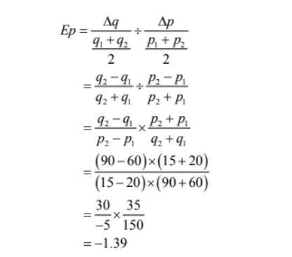
| Price of commodity X | Quantity demanded of X | Point |
| 20 | 60 | A |
| 15 | 90 | B |
The above table is represented in the following Diagram 3.7.


C) Arc elasticity of demand: In the above measure we have studied the measurement of elasticity at a point on a demand curve. When elasticity is measured between two points on the same demand curve, it is known as arc elasticity.
According to Prof. Baumol, “Arc elasticity is a measure of the average responsiveness to the change in price exhibited by a demand curve over some finite stretch of the demand curve.”. Any two points on the same demand curve make an arc shows the arc elasticity of demand.
In other words, arc price elasticity of demand measures elasticity of demand at two points on the demand curve.
D) Geometrical measure of elasticity of demand: If there is a linear demand curve the point elasticity of demand is measured by geometrical method i.e. it is the ratio of lower segment of the demand curve below the point to the upper segment of the demand curve above the point on the demand curve.
Symbolically,
Ep = Lower segment of the demand curve below the point
Upper segment of the demand curve above the point
The geometric method can be explained through the
Diagram 3.8 given below:

6) Discuss the different degrees of elasticity of demand.
Answer : Different commodities have different elasticities of demand. Some commodities have more elastic demand then others, while other commodities have relative elastic demand. The elasticity of demand ranges from zero to infinity (0-∞). It can be equal to zero, one, less than one, greater than one and equal to unity.
“The degree of responsiveness to the change in demand in a market for a commodity is great or small, as the amount demanded increases much or little for a given fall in price and diminishes much or little for a given rise in price of the commodity”.
The various level or the degree of elasticity of demand is explained in brief below:
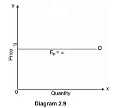
- Perfectly elastic demand (Ep = ∞): The demand is said to be perfectly elastic, if slight change in price leads to infinite change in the quantity demanded of the commodity. In other words, it is the level of responses where the consumer is able to buy all the available commodity at a particular price where the demand is elastic. The demand curve under this situation is horizontal straight line parallel to X axis shown in the Diagram 3.9 below.
This type of demand curve is relevant in perfect competition. But in the real world, this case is exceptionally rare and are not of
any practical interest.
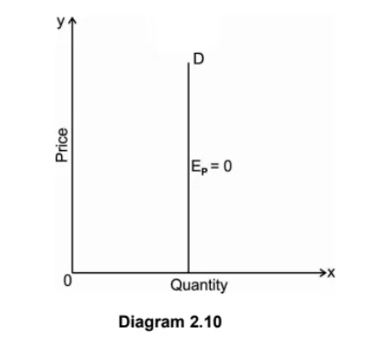
- Perfectly inelastic demand (Ep = 0): The demand is said to be perfectly inelastic, if the demand for a commodity does not change with a change in price of the commodity. In other words, the perfectly inelastic demand of a commodity is opposite to the perfectly elastic demand. Under the perfectly inelastic demand, a rise or fall in price of a commodity the quantity demanded for a commodity remains the same. The elasticity of demand will be equal to zero. The demand curve is vertical straight line parallel to Y-axis shown in the Diagram 2.10.
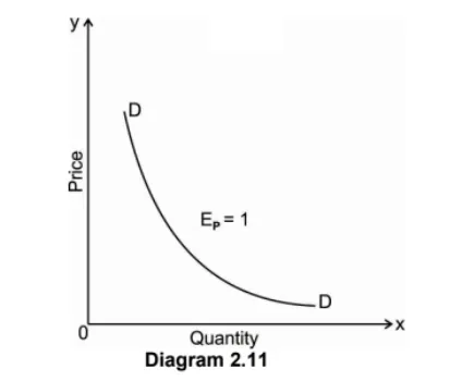
- Unitary elastic demand (Ep = 1): Demand is said to be unitary elastic when the percentage change in the quantity demanded for a commodity is equal to the percentage change in its price. The numerical value of unitary elastic of demand is exactly equal to one i.e. Marshall calls it as unit elastic. The demand curve is rectangular hyperbola shown in the Diagram 2.11.
- Relatively Elastic demand (Ep> 1): Demand is said to be relatively elastic, when the percentage change in quantity demanded of a commodity is greater than the percentage change in its price. In other words, it refers to a situation in which a small change in price leads to a great change in quantity demanded. The demand curve under this situation is flatter as shown in Diagram 2.12. Such demand curve is seen under monopolistic competition.

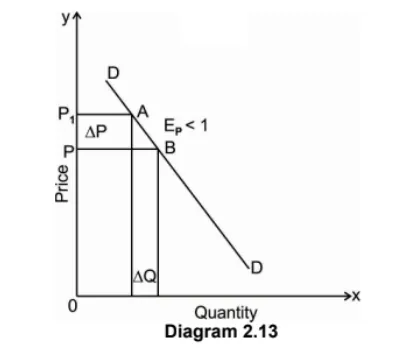
- Relatively Inelastic demand (Ep< 1): Demand is relatively inelastic when the percentage change in the quantity demanded of a commodity is less than the percentage change in the price of the commodity. The demand curve under this situation is steeper shown in Diagram 2.13. Such demand curve is observed under monopoly market.
7) What are the factors affecting price elasticity of demand?
Answer: The price elasticity of demand depends upon number of factors which affects its elasticity. They are as follows:
a) Nature of goods or commodity: The elasticity of demand for a commodity depends upon the nature of the commodity,
i.e., whether the commodity is a necessary, comfort or luxury good.
The elasticity of demand for a necessary commodity is relatively small. For example, if the price of such a good rise, its buyers generally are not able to reduce its demand as its necessity commodity. The elasticity of demand for a luxury good is usually high.
This is because the consumption of a such good, unlike that of a necessary commodity, can be delayed. That is why if the price of such a commodity increase, the demand for the good can be significantly reduced.
b) Availability of Substitute Goods: The price elasticity of demand also depends upon the substitution of goods. If there is a close substitute for a particular commodity in the market, then the demand for such commodity would be relatively more elastic. For example, since tea and coffee are close substitute for each other in the commodity market, a rise in the price of coffee will result in a considerable fall in its demand and a consequent rise in the demand for tea. Therefore, a demand for coffee will be relatively more elastic because of the availability of tea in the market.
c) Alternative and Variety of Uses of the Product: as we know that the resources have an alternative use. The demand for such goods has many uses. The more the alternative and variety of uses of a good, the more would be its elasticity of demand. For example, Electricity is used for many purposes such as lighting, heating, cooking, ironing and also use as a source of power in many industries & households. That is why
when the price of electricity increases, its demand will decrease and vice versa.
d) Role of Habits and custom: if the consumer has a habit of something, he will not reduce his consumption even if the price of such commodity increases the demand for them do not decreases considerably and so their elasticity of demand will be inelastic.
Ex; Alcohol, Cigarettes which are injurious for health but people still consume it because of their habit.
e) Income Level of the consumer: The elasticity of demand differs due to the change in the income level of the households.
Elasticity of demand for a commodity is low for higher income level groups then the people with low incomes. This is because rich people are not influenced much by changes in the price of goods. Poor people are highly affected by the increase or decrease in the price of goods. As a result, demand for the lower income group is highly elastic in demand.
f) Postponement of Consumption: if the consumer postponed the consumption of commodity in future the demand is relatively elastic. For example, commodities whose demand is not urgent, have highly elastic demand as their consumption can be postponed if there is an increase in their prices. However, commodities with urgent demand like medicines have inelastic demand because it is an essential commodity whose
consumption cannot be post pended.
g) Time Period: Price elasticity of demand is related to a period of time. The elasticity of demand varies directly with the time period. In the short run the demand is generally inelastic and in long-run it becomes relatively elastic. This is because consumers find it difficult to change their habits, in the short run, in order to response to the change in the price of the commodity. However, demand is more elastic in long run as
their other substitutes available in the market, if the price of the given commodity rises.
8) Write a note on:
Answer : a) Income elasticity of demand.
As we have discussed earlier the factor which determines elasticity of demand for a commodity. The consumer’s income is one of the important determinants of demand for a commodity. The demand for a commodity and consumer’s income is directly related to each other, unlike price-demand relationship. Income elasticity of demand shows the degree of responsiveness of quantity demanded of a commodity to a small change in the income of a consumer.
In other words, the degree of responsiveness of quantity demanded to a change in income is measured by dividing the proportionate change in quantity demanded of a commodity by the proportionate change in the income of a consumer.
Percentage change in purchases of a commodity Income Elasticity = Percentage change in income
b) Cross elasticity of demand.
Sometimes we find two goods are inter-related to each other either they are substitute goods or commentary goods. Cross elasticity of demand measures the degree of responsiveness of demand for one good in responsive to the change in the price of another good.
Percentage change in quantity demanded of commodity ‘X’ E =
Percentage change in the price of commodity ‘Y’
Classification of goods based on value of cross elasticity of demand:
a. Substitution: If the value of elasticity between two goods are positive the goods are said to be substitute to each other. For
example, Tea and coffee, if the price of tea increases the demand for coffee increases.
b. Complementary: if the value of elasticity between two goods are negative the goods are said to be complementary. For
example, car and petrol, if the price of petrol increases the demand for car decreases.
c. Unrelated: if the value of elasticity between two goods are zero then the goods are said to be unrelated to each other. For
example, table and car, if the price of table increases there is no change in the demand for car.
c) Promotional elasticity of demand.
It is also known as ‘Advertisement elasticity’. In modern times an increase in expenditure on advertisement or promotion leads to an increase in the demand for a commodity Promotional elasticity of demand is the proportional change in quantity demand due to proportionate change in promotional expenditure. In other words, percentage change in the quantity of demand for a commodity divided by the percentage change in promotional expenditure shows the promotional elasticity of demand.
Percentage change in quantity demanded E
Percentage change in advertisement expenditure
The greater the elasticity of demand, its better for a firm to spend more on promotional activities. The promotional elasticity of
demand is usually positive.
9) Explain the concepts of revenue in detail.
Answer : The term revenue refers to the income obtained by a firm or a seller through the sale of commodity at different prices.
The revenue is classified as:
- Total revenue: The total revenue or income earned by a firm or producer from the sale of the output he produced is called the total revenue. Thus, the total revenue is the price multiply the quantity of output.
TR = P×Q
Where,
TR = Total Revenue.
P = Price of a commodity.
Q = Total Output sold.
Thus, Total revenue is the sum of all sales, receipts or
income of a firm in the market. - Average revenue: The average revenue refers to the revenue obtained by the firm by selling the per unit of output of a commodity. It is obtained by dividing the total revenue by total unit of output sold in the market.
AR = TR
Q
Or
AR = P
Where, AR= Average revenue.
The average revenue curve shows that the price of the firm’s product is the same at each level of output. In other words, the average revenue curve of a firm is also the demand curve of the consumer.
- Marginal revenue: Marginal revenue is the additional revenue earned by selling an additional unit of the commodity. In other words, Marginal revenue is the change in total revenue due to the sale of one additional unit of output. Thus, marginal revenue is the addition commodity made to the total revenue by selling one more unit of the commodity. In algebraic terms, marginal revenue is the net addition to the total revenue by selling n units of a commodity instead of n – 1.
Thus, MRn = TRn – TRn-1
Or
MR = ΔTR
ΔQ
Relationship between price elasticity and total revenue: Elasticities of demand can be divided into three broad categories: elastic, inelastic, and unitary. An elastic demand is one in which the elasticity is greater than one, indicating a high responsiveness to changes in price. Elasticities that are less than one indicates low responsiveness to price changes and correspond to inelastic demand. Unitary elasticities indicate proportional responsiveness of either demand or supply, as summarized in the following table:
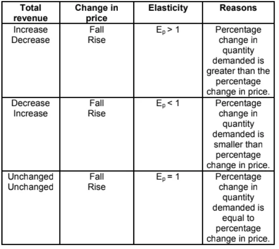
The relationship between the price elasticity and total revenue shows the following analysis from the above table.
A. When demand is elastic, price and total revenue move in opposite directions.
B. When demand is inelastic, price and total revenue moves in same direction.
C. When demand is unitary elastic, total revenue remains unchanged with the price changes.
This relationship can be easily understood by the following diagram: 2.14
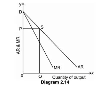
Relationship between price elasticity and Average revenue and Marginal revenue: The relationship between AR, MR and elasticity of demand is very useful to understand at any level of output. This relationship is also very useful to understand the price- determination under different market conditions. It has been discussed that average revenue curve of a firm is the same thing as the demand curve of the consumer for the product of the firm under market.
Pingback: FYBCOM Economics Sem 1 Chapter 1 Notes | FYBAF | FYBMS | Mumbai University - University Solutions